Graph_Convolutional_Networks (GCN)_001 _ Understanding the GCN Formula Step by Step

---

Introduction

In this post, we will break down the fundamental Graph Convolutional Network (GCN) formula with a simple example. We will walk through each component, including the adjacency matrix, degree matrix, normalization, and feature transformations. By the end of this lesson, you’ll have a clear understanding of the basic mathematical operations behind GCNs.

 

In a Graph Convolutional Network (GCN), the key transformation is given by the following formula:

 

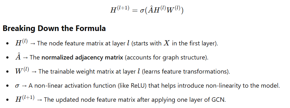
Now, let's go step by step to understand how each part of this formula works in practice.

---

 

Step 1: Understanding the Graph Structure

Consider a simple graph with three nodes:

   (1) -- (2)
     \    /
      \  /
       (3)

The adjacency matrix (A) represents the connections between nodes:

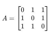
• The rows and columns correspond to nodes.
• A value of 1 indicates a connection between nodes, while 0 means no direct connection.

Step 2: Adding Self-Loops

We add self-loops to each node by introducing an identity matrix (I):

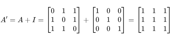
Now, each node is also connected to itself.

---

Step 3: Computing the Degree Matrix

The degree matrix (D’) is a diagonal matrix where each diagonal element represents the sum of connections for that node:

For our graph, each node is connected to two other nodes and also has a self-loop (since we added the identity matrix I). So, each node has a total of 3 connections.

Why are only diagonal elements nonzero?

• The degree matrix is always diagonal because it only counts the number of edges per node — not their relationships with other nodes.
• The off-diagonal elements are always zero because they do not represent any direct connection count, only the total degree of each node.
• Row 1: Node 1 is connected to Node 2, Node 3, and itself → Total = 3
• Row 2: Node 2 is connected to Node 1, Node 3, and itself → Total = 3
• Row 3: Node 3 is connected to Node 1, Node 2, and itself → Total = 3

Thus, the degree matrix is:

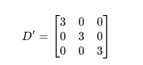
Each diagonal element (3) represents the sum of connections for that node, and of

---

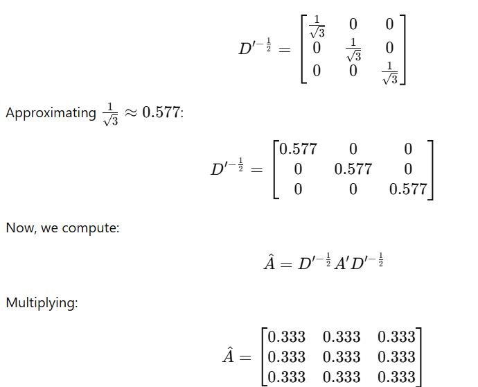
Step 4: Normalizing the Adjacency Matrix

We compute the inverse square root of the degree matrix:

 

Step 5: Applying Features 

At this stage, we introduce the feature matrix X, which represents the features of each node in our graph.

What is the feature matrix X?

• Each row in X corresponds to a node in our graph.
• Each column in X represents a feature associated with the node.
• The values in X are imaginary/random for this example and do not represent real-world data. They are just chosen to make the calculations clear.

Assume we have 3 nodes, and each node has 2 features (e.g., some numerical properties like “height” and “weight” in a social network or “temperature” and “humidity” in a sensor network).

We define our feature matrix X as follows:

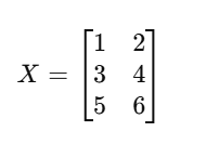
Here’s what each value represents:

• Node 1: Feature 1 = 1, Feature 2 = 2
• Node 2: Feature 1 = 3, Feature 2 = 4
• Node 3: Feature 1 = 5, Feature 2 = 6

Important Notes:

• These values are arbitrary and just for illustration. In real applications, these features could represent anything from user preferences in a social network to pixel values in an image.
• The number of columns in X (here, 2) represents the input feature dimension — it defines how many numerical properties each node has.

Now that we have our feature matrix, the next step is to apply the graph convolutional operation using weights.

 

Step 6: Multiplying with A^ (Normalized Adjacency Matrix)

Now that we have our feature matrix X, the next step is to perform the graph convolution operation by multiplying X with the normalized adjacency matrix A^(A- hat).

What is A^?

• A- hat is a modified version of the adjacency matrix that includes self-loops as described in previous steps
• It helps in aggregating information from each node’s neighbors including itself.
• The purpose of multiplying with A-hat is to allow nodes to receive feature information from their neighbors.

For our example, the multiplication looks like this:

What does this multiplication do?

• It aggregates features from neighboring nodes.
• Since each node has 2 direct neighbors (plus itself), the sum results in (3,4) for each row.
• This shows that every node’s updated feature is influenced by the sum of itself and its neighbors’ features.

---

Step 7: Applying the Weight Matrix W

Now, we introduce the weight matrix W, which is a trainable parameter in a GCN:

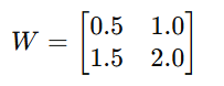
• These numbers are random and do not come from real data. They are just used for illustration purposes.
• In a real GCN, these numbers are initialized randomly and then updated during training using backpropagation.

What is the Weight Matrix W?

• W is a matrix that transforms the feature representations of nodes.
• It learns to extract meaningful patterns from node features over time.
• Each element in W represents how important a particular input feature is in transforming node embeddings.
• W is learned during training and helps in transforming the features into a new space.
• The rows in W correspond to the input feature dimension (2 features per node in X).
• The columns in W correspond to the new transformed feature dimension (which could be different).

How are the values in W selected in real applications?

• Initially, they are set randomly (e.g., small random values close to zero).
• As the model trains, an optimization algorithm (like Gradient Descent) adjusts these values to minimize the loss.
• Over time, W learns to capture the important relationships between node features and their labels (or other predictive targets).

Step 8: Understanding the Final Transformed Features

At this point, each node’s features have been updated based on:

1. Its own features (from X)
2. The features of its neighbors (aggregated using A-hat)
3. The learned transformation (from W)

Key Takeaways

• The graph convolution operation allows each node to gather information from its neighbors.
• The weight matrix W helps the model learn patterns in the data.
• The output matrix represents the new features for each node, which can now be used for classification, clustering, or further graph learning tasks.

Step 6: Applying the Activation Function

Conclusion: Summary of Graph Convolutional Operation

1. Start with the feature matrix X, where each row represents a node’s features.
2. Multiply X with the normalized adjacency matrix A-hat(A^), aggregating neighboring node information.
3. Multiply the result with a trainable weight matrix W to transform features.
4. (Optional) Apply an activation function like ReLU for non-linearity.
5. Use the new features for tasks like node classification or link prediction.

In this post, we broke down the GCN formula step by step, starting with the graph structure and progressing through normalization, feature transformation, and activation. In the next lesson, we will implement this mathematically defined GCN as a simple model in PyTorch (included in pytorch beginner catogory).